Scientific Report 1155
This report is also available as a PDF document .
Abstract
As part of the GEF Loan 1155 project, this study aims to model the structure and estimate the above-ground biomass (AGB) of dry Miombo woodlands in Namibia using a combination of field data and remotely sensed data.
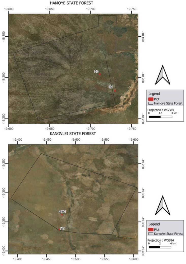
Data were collected in four plots (50 m x 100 m) in the Hamoye and Kanovlei state forests in the province of Kavango East, northeast Namibia. The locations of GEDI spaceborne LiDAR footprints were used to guide plot location, to maximise overlap with satellite observations.
Fieldwork took place in March 2023, employing a Riegl VZ-1000 terrestrial laser scanner (TLS) to capture detailed vertical foliage profiles. Scans were distributed in a 25 m x 25 m grid to minimise occlusion in the relatively open Miombo understorey. The precise geographic coordinates of the plots were determined using a GNSS receiver for accurate georeferencing within the global coordinate system.
This research addresses a key knowledge gap regarding the effectiveness of TLS data in discriminating woody plant growth forms between the understorey and overstorey layers, modelling vertical structure, and estimating AGB in dry woodland ecosystems.
Background
Miombo woodlands, one of the most expansive ecosystems in sub-Saharan Africa, are distinguished by an open tree canopy, a discontinuous understorey of shrubs and small trees, and a continuous, grass-dominated ground layer 1 2 3. These woodlands are shaped by a combination of environmental factors, including precipitation, fire, and wildlife activity. Based on mean annual precipitation (MAP), Miombo woodlands are broadly classified into wet Miombo (MAP above 1000 mm) and dry Miombo (MAP below 1000 mm). Although often overlooked in research, the understorey layer, consisting of small trees, shrubs and saplings of larger trees, plays a crucial role in nutrient cycling, biodiversity, and regeneration within these ecosystems. Most research has focused on larger trees comprising the overstorey vegetation, leaving the understorey relatively understudied.
This study focuses on dry Miombo woodlands in Namibia, which receive less than 700 mm of annual precipitation and experience frequent fire disturbances. The project aims to evaluate the effectiveness of terrestrial laser scanning (TLS) in characterizing various growth forms including shrubs, saplings, and large trees, to model stand structure and above-ground biomass (AGB) in these dry woodlands. Tree segmentation within plots and wood and leaf separation are achieved through quantitative structural models (QSMs), enabling the estimation of crown dimensions and tree volume, which are converted into AGB estimates using species-specific wood density values.
The primary objectives of this project are to:
- Assess the accuracy of AGB estimates derived from allometric in situ measurements (stem diameter and height) compared to TLS-derived volumetric models,
- Describe the vertical structure of the woodland, and
- Estimate the total, understorey, and overstorey AGB based on TLS data.
Field surveys were conducted in the Hamoye and Kanovlei state forests of Namibia. These plots represent typical dry woodland conditions, making them ideal for assessing AGB through TLS in dry Miombo woodlands. The data collection took place in March 2023.
For this research, the following equipment was borrowed under GEF Loan 1155: Riegl VZ-1000 terrestrial laser scanner, Global Navigation Satellite Systems (GNSS) receivers, Tripods, and Reflectors.
Survey procedure
The initial plan was to scan six 1-hectare plots (three in Kanovlei and three in Hamoye). However, due to delays caused by customs and equipment failures, TLS measurements were conducted on four half-hectare plots (100 m x 50 m): SK1 and K1 in Kanovlei, and H1 and H3 in Hamoye. The scans were carried out using a Riegl VZ-1000 terrestrial laser scanner, with four transects set up for each plot–three inside the plot boundaries and one outside (see Figure 2).
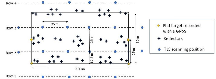
At eight scanning positions along Rows 2 and 3, located inside each plot, the vegetation was scanned with the scanner in both horizontal and vertical orientation, to capture the canopy structure. In Rows 1 and 2, scanning was conducted only in the horizontal direction, with the purpose of minimising shadow effects and maximising spatial coverage of vegetation within the plot. Reflectors used as tie-points for aligning scans, were placed at various locations within each transect, including the corners of the plots (Figure 3A). Due to a limited number of reflectors, some were repositioned from the edges between Rows 3 and 4 before scanning commenced.
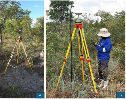
The distance between each scan position was approximately 25 meters, though distance varied based on vegetation density and the visibility of reflectors at each location. To ensure accurate georeferencing, a GNSS base station was set up on a tripod in an open area near the southwestern corner of each plot. The GNSS rover, with its antenna mounted on tripods at the plot corners, was used to record precise plot corner locations. Corner locations were saved when the Geometric Dilution of Precision (GDOP) was below 2, with each corner taking approximately 5-10 minutes to record. The identification of targets as common anchor points served as ground control points and enabled to align point clouds within a subplot 4.
In addition to TLS data, understorey (stem diameter < 5cm and height > 50 cm) and overstorey trees (stem diameter 5 cm) were measured. The overstorey vegetation was measured within the entire plot following the SEOSAW protocol v3.6 (https://seosaw.github.io/manuals.html) while the understorey vegetation was measured within 5 subplots of 25 m x 25 m. The following attributes were measured for the woody vegetation:
- Name of species,
- Stem location, using XY coordinates,
- Stem diameter, measured with a Vernier calliper at 0.1 cm height for the understorey plants and at 1.3 m with a diameter tape for the overstorey plants,
- Crown diameter in two perpendicular directions (crowns 1 and 2),
- Height measured by using a laser rangefinder or a DBH pole,
- Status including dead and resprouting stems,
- Cause of damage
Challenges and Recommendations
Two primary issues were encountered during TLS data collection:
- Frequent software crashes: The laptop and scanning software crashed during scanning, especially when the scan completion percentage exceeded 90%.
- Battery failures: Scanning often stopped prematurely when the battery was low, further delaying the process.
For future borrowers working in tropical regions, it is recommended to use a high-performance laptop capable of withstanding high temperatures and extended operation. Adequate power backups and reliable battery solutions are essential to avoid interruptions during scanning.
Data quality
Data were collected using standardized protocols to minimize errors. The following factors contributed to the overall quality of the data:
- Precision of GNSS Measurements: The GNSS measurements were recorded when the GDOP was below 2, ensuring high positional accuracy. This was crucial for georeferencing the plots and aligning TLS data.
- Sampling Strategy: A 25 m x 25 m sampling grid was employed to minimize occlusion effects,
The TLS data were evaluated based on the following criteria:
- Scan Density and Coverage: To capture comprehensive data on the canopy structure, scanning was conducted in two directions. This multidirectional scanning improved the density and accuracy of the point cloud data.
- Reflector Visibility: The use of multiple reflectors placed throughout the plot ensured good alignment and registration of scans. The strategic placement of reflectors minimized potential data gaps.
For the GNSS positioning, reference station point KP2 were processed using the online Trimble RTX service. Rover points GPS05,06,07 and 08 processed in Leica Infinity using a Phase Fixed solution. Errors within the GNSS receiver tolerance (1cm plan, 2cm vertical). Coordinates exported in UTM Zone 34 South.
Processing and modelling
The TLS data collected in the field were processed using RiSCAN PRO software to create a coherent point cloud for each plot. Initial scan registration was achieved using reflectors placed across each plot, and further refinement was conducted via a Multi-Station Adjustment to optimize alignment and minimize errors in the point cloud data. The standard deviation of the registrations was maintained within an acceptable range, ensuring high accuracy for further analysis.
Concerning the Point cloud Processing, the details for each plot are as follows:
- Plot H1: Scans were registered initially using targets, then refined using a Multi-Station Adjustment in RiSCAN PRO v2.7. The standard deviation of the registration was 0.0766 m. However, ScanPos001 and ScanPos012 could not be registered due to insufficient overlapping targets, and ScanPos016 to ScanPos021 had no scanned targets, leading to incomplete data for those positions.
- Plot H3: Scans were successfully registered using targets and further refined with a MultiStation Adjustment in RiSCAN PRO v2.7. The standard deviation was 0.0161 m, indicating good quality registration.
- Plot K1: This plot could not be processed due to insufficient overlap between target locations, which resulted in incomplete alignment of the scans. Consequently, the data in this directory are not geo-referenced, and each scan position is located at coordinates (0, 0, 0).
- Plot SK2: Scans were registered using targets and refined with a Multi-Station Adjustment in RiSCAN PRO v2.7. The standard deviation for this plot was 0.0439 m, reflecting accurate alignment and registration.
Data Conversion and Export
The raw TLS data were converted into the standard LAS format, a widely accepted format for point cloud data, using RiSCAN PRO. This step ensured compatibility with post-processing tools in R and Python, enabling flexible data manipulation for further analyses. LAS files were exported with georeferenced coordinates in UTM Zone 34S to ensure accurate spatial alignment with GNSS-measured plot boundaries.
Vertical Structure Analysis
The vertical structure of the plots was analyzed using R with the lidR and rLiDAR packages. The point clouds were first filtered to separate ground points from non-ground points. A digital terrain model (DTM) was created to establish a ground reference, and a canopy height model (CHM) was derived by subtracting the DTM from the canopy points. The canopy was divided into layers, such as understorey and overstorey, and the vertical profile was analyzed by computing vegetation height metrics, including mean and maximum canopy height. These metrics provide insights into the vertical structure of the woodland.
Preliminary findings
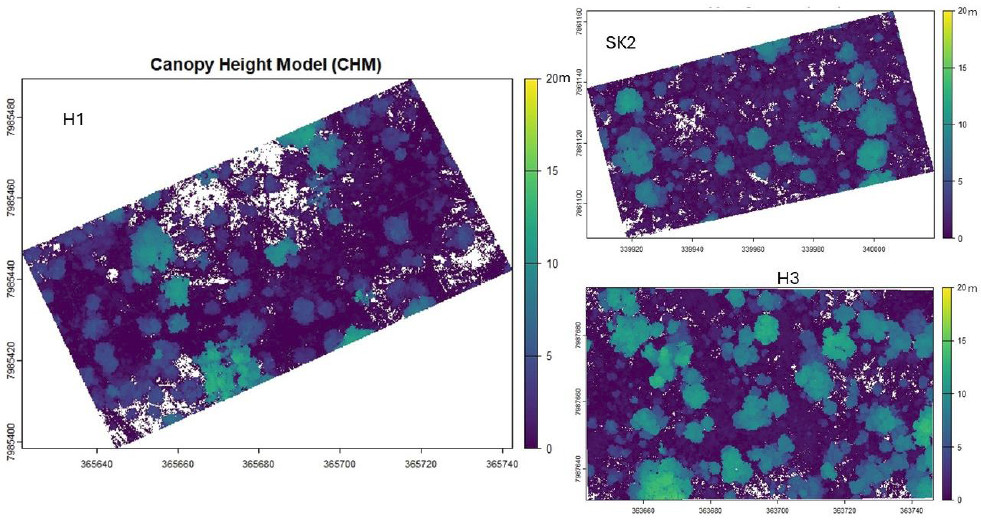
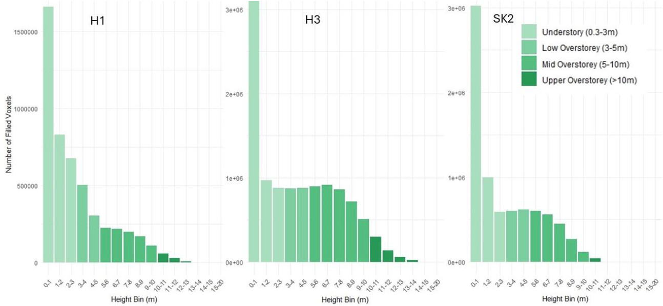
In our preliminary findings, we present the canopy density profile and the Canopy Height Model (CHM) for the study plots. The canopy density profile was generated by classifying canopy height into 1-meter increments, excluding heights below 30 cm (Fig. 5). This profile highlights distinctive canopy structure characteristics across the three plots: H1, H3, and SK2.
In Hamoye, plot H1 shows a relatively low mean canopy height (2.19 m) and median height (1.57 m), suggesting a predominantly low canopy structure. In contrast, plot H3 in Hamoye exhibits the highest mean and median canopy heights (3.71 m and 3.12 m, respectively), with a maximum height reaching 15.15 m, which indicates a taller canopy with potentially more developed vegetation. Plot SK2 in Kanovlei lies between these two, with a mean height of 2.84 m and a median height of 1.85 m, suggesting a mixed canopy structure that includes both low and midheight vegetation. These structural differences may reflect variations in environmental conditions and disturbance histories across the plots.
Additionally, a CHM was generated to visualize the spatial distribution of canopy heights and tree coverage within each plot (Fig. 4), providing further insight into the vertical forest structure.
Conclusions and recommendations
This study demonstrates the effectiveness of Terrestrial Laser Scanning (TLS) in capturing detailed canopy profiles within Miombo woodlands. Next steps will involve estimating aboveground biomass (AGB) across canopy layers and exploring TLS’s potential for identifying individual trees across different growth forms, further enhancing our understanding of forest structure and dynamics.
For future field work, implementing a dense reflector placement strategy and optimizing GNSS to lower GDOP values could further improve data alignment and accuracy.
Location of the archived data
The data from this research will be archived on a public data repository, such as Zenodo or Edinburgh Data Share, where it will be accessible with a DOI. This archiving will occur following the publication of research results, ensuring that the data is freely available to the scientific community and general public for further analysis and application.
Publications (including conference presentations)
Title: Characterizing Growth Forms and Estimating Biomass in Dry Miombo Woodlands Using Terrestrial Laser Scanning
Status: In progress
Expected Submission: 2025
Target Journal: GIScience & Remote Sensing
References
-
Frost, Peter. 1996. “The Ecology of Miombo Woodlands.” Pp. 1157 in The Miombo in transition: Woodlands and Welfare in Africa. Bogor, Indonesia: Centre for International Forestry Research. ↩
-
Mayaux, Philippe, Etienne Bartholomé, Steffen Fritz, and Alan Belward. 2004. “A New Land cover Map of Africa for the Year 2000.” Journal of Biogeography 31(6):86177. doi: 10.1111/j.1365-2699.2004.01073.x. ↩
-
Ryan, Casey M., Timothy Hill, Emily Woollen, Claire Ghee, Edward Mitchard, Gemma Cassells, John Grace, Iain H. Woodhouse, and Mathew Williams. 2012. “Quantifying Smallscale Deforestation and Forest Degradation in African Woodlands Using Radar Imagery.” Global Change Biology 18(1):24357. doi: 10.1111/j.1365-2486.2011.02551.x. ↩
-
Wilkes, Phil, Alvaro Lau, Mathias Disney, Kim Calders, Andrew Burt, Jose Gonzalez de Tanago, Harm Bartholomeus, Benjamin Brede, and Martin Herold. 2017. “Data Acquisition Considerations for Terrestrial Laser Scanning of Forest Plots.” Remote Sensing of Environment 196:14053. doi: 10.1016/j.rse.2017.04.030. ↩
