Rift propagation for ice-sheet models (RIP-ICE)

Scientific Report 1149

This report is also available as a PDF document .

Abstract

The credibility of sea level rise projections is undermined by large uncertainties that are due to model treatments of ice shelves - the floating extensions of ice sheets which constrain the flow of ice from the interior to the ocean. Assuming that ice shelves will disintegrate leads to a much higher estimate of ice discharge than assuming they remain in place. No forecast so far, however, has included the processes of ice fracture and rift propagation that lead to ice shelf disintegration. These processes disrupt the normal assumptions of continuity inherent in ice sheet models and are highly dependent on the heterogeneous nature of ice shelves. Here, we report the results from multiple transient electromagnetic soundings integrated with ground-penetrating radar (GPR), active-source and borehole geophysical data, spanning 10 km across a suture zone of Larsen C Ice Shelf (LCIS), Antarctica. Our results indicate the presence of two ice-shelf layers. The uppermost layer, ~300 m thick, has resistivity 103-106 m. We interpret this layer as meteoric ice. The base of the uppermost layer coincides with a concentration of radar reflectors and the documented ice shelf base. Yet, our results reveal the presence of a lower shelf layer 25-56 m thick with resistivity 3-20 m interpreted as permeable basal marine ice. This reconstruction agrees closely with modelled marine-ice thicknesses in the area. The porosity of this layer is 0.18-0.40, higher than measured farther downflow, suggesting the layer consolidates once formed. These heterogeneities in ice shelf properties should be accounted for in future models of fracture development and propagation in the LCIS, and implied assessments of its future stability.

Background

Marine ice is important for many reasons including basal mass budget of ice shelves, and its influence on rheology and stability (Craw, 2023¹). Suture zones are present in all large and numerous smaller Antarctic ice shelves, stabilising them by delaying the opening of rifts that propagate quickly through meteoric ice units derived from tributary glaciers (Khazendar et al., 2009², Kulessa et al., 2014³, 2019⁴, Jansen et al., 2015⁵). Basally-accreted marine ice within suture zones contains seawater and is warmer than surrounding meteoric ice, allowing suture zones to arrest rifts by accommodating strain and delaying or preventing brittle fracture (Kulessa et al., 2019⁴). For example, marine ice is well known to play a crucial role in stabilising the Larsen C Ice Shelf (LCIS), Antarctic Peninsula (Kulessa et al., 2014³). However, a recent study by Harrison et al. (2022)⁶: shows that ocean warming significantly reduces the extent and thickness of LCIS’s marine ice, with potential implications for the shelf’s future stability. There is an urgent need for measurements that are feasibly acquired and not only capable of diagnosing the presence of basal marine ice, but also of characterising its depth, thickness and physical properties such as porosity and seawater content (Killingbeck et al., in review⁷).

Electromagnetic (EM) techniques measure subsurface electrical resistivity structure and have been used successfully on glaciers to detect subglacial water (e.g., Mikucki et al., 2015⁸, Killingbeck et al.2020⁹), and on sea ice to detect and quantify sub-ice platelet layers (SIPLs) (e.g., Hunkeler et al., 2016¹⁰, Brett et al., 2020¹¹, Haas et al., 2021¹²). Basal marine ice also forms by accretion of ice crystals from supercooled water onto the underside of an ice shelf, resulting in a lower shelf layer that is porous and permeable with interconnected brine channels (Craven et al., 2005¹³, 2009¹⁴, 2014¹⁵). It is therefore reasonable to assume that such permeable marine ice will have bulk electrical resistivity values that range between highly-resistive meteoric shelf ice (> 10000m; Kulessa, 2007¹⁶) and highlyconductive seawater (0.36 m; Nicholls et al., 2012¹⁷). Similarly, we also expect to be able to diagnose the porosity of permeable basal marine ice from measured electrical resistivities using conceptual frameworks established for sea ice (e.g. Gough et al., 2012¹⁸; Langhorne et al., 2015¹⁹; Haas et al., 2021¹²).

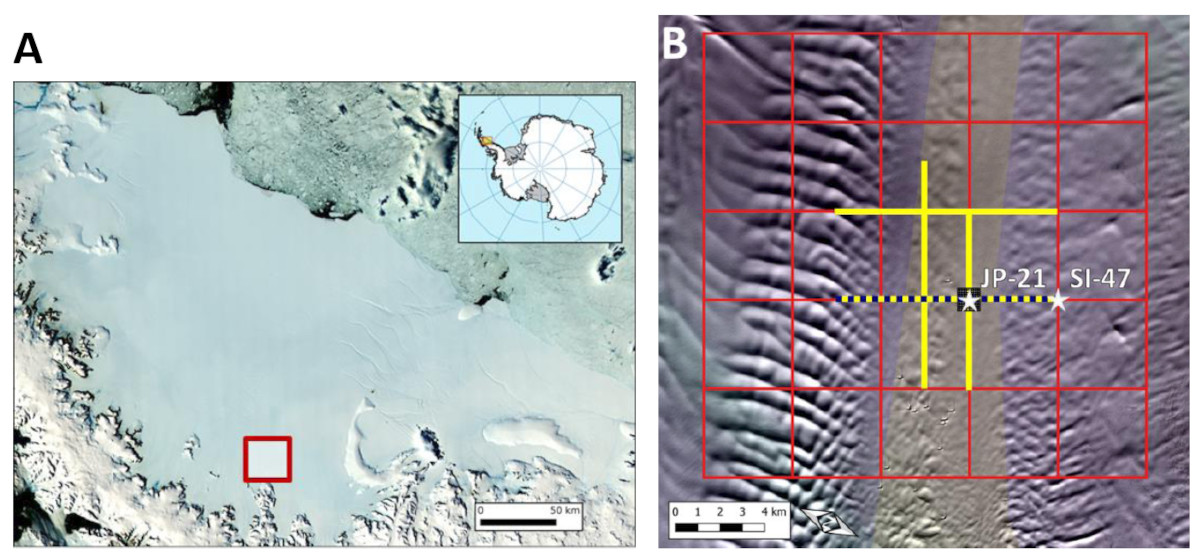
Here we present the results of an integrated geophysical survey acquired in the 2022/23 austral summer on the Joerg Peninsula suture zone, LCIS (Fig. 1). The survey, which aimed to investigate the thickness and electrical resistivity of the permeable basal marine ice layer, combined surfacebased transient electromagnetics (TEM), ground-penetrating radar (GPR) and active source seismics with borehole televiewer, sonic and electrical logs. Resistivity is used to infer the porosity and its spatial variability across the permeable basal marine ice layer. To support the field measurement program, GEF kindly issued a loan of the following:

• Sensors and Software Pulse EKKO PRO GPR system with 25, 50, 100 and 200 MHz antennas, including the high-power (1000 V) transmitter and the multi-channel adapter.
• Two Leica VIVA GS10 Professional GNSS Receivers, and Leica GeoOffice software, to facilitate GPR line positioning.
• Geonics PROTEM 47 Transmitter and 58 Receiver, 3D High Frequency coil and Interpex IX1D Software.

Figure 1. A Larsen C Ice Shelf (LCIS), with location in Antarctica shown in the inset, and red rectangle indicating the field site in B. The background is a MODIS scene from August 2016. B Joerg Peninsula suture zone showing the location of two boreholes (white stars, labelled JP-21 and SI47) with a seismic survey also conducted at the JP-21 star location, the planned long-line (red, squares spaced 4 4 km) and high-resolution (black grid underlying JP-21 star, squares spaced 100x100 m in a 1x1 km grid) GPR grids, the actual long-line GPR data recovered (yellow lines) and the profile of 21 TEM soundings spaced 500 m apart (blue dotted line). The coordinates of the start of the TEM profile are -67.958191°, -64.432125°, and the end of the profile are -68.041545°, 64.325607° (coincident with the location of borehole SI-47). The coordinates of the JP-21 borehole location are -68.008614°, -64.367714°. The coastline and grounding line in A and background in B are from the MEaSUREs MODIS Antarctic mosaic (Haran et al., 2018²⁰).

Survey procedure

Transient Electromagnetics (TEM)

TEM data were acquired with the GEF-supplied Geonics PROTEM47 system consisting of a threechannel digital time-domain receiver unit, a three component multi-turn receiver coil (area 31.4m²), and the TEM47 battery-powered transmitter. A 100x100m square transmitter loop was laid out and the receiver coil was placed in the center of the square. Laying out and recovering the transmitter loop required a bit of practice and adaptation of the GEF equipment. The latter came in eight 50 m sections on eight separate and awkward cable reels. We took the eight cable sections off the reels and connected the sections together with electrical tape, and then spooled the 400 m long resulting cable onto a spare larger cable reel. The latter was then deployed on the back of a Siglin sledge and with the operator sitting on a Zarges box on the sledge next to the large reel. The cable could then be reeled out and in with ease, with the sledge being towed by snowmobile driven at an appropriate speed. However, stretching the cable during the process frequently resulted in cable sections coming apart, which was not always obvious and a lot of time was consequently spent by the fieldworkers walking along the 400 m cable to find the fault.

Figure 2. Visual representation of typical deployment of a TEM station in Antarctica, as described in the text. Central image taken by photogrammetry drone, showing 100x100 m square transmitter loop and central receiver. The four corners and centre position are marked by flags, with central flag taken down during data acquisition to avoid possible electric interference with TEM measurements during windy conditions. Top left image (credit: D. Prior) shows receiver loop deployment using 400 m cable spooled off a reel, bottom left image shows the transmitter and top right and bottom right images show 3-D receiver loop and recording system

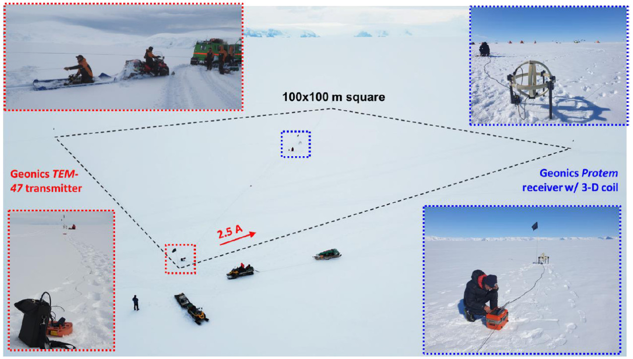
We would therefore recommend that a 400 m long cable be used in the future, instead of 8 separate sections. It is also useful to deploy a set of five flags prior to TEM equipment deployment, one at the centre point where the receiver coil is located, and one at each corner of the 4x100 transmitter loop. This is best achieved by pre-planning flag locations using PC-based GIS software and storing the resulting coordinates in a hand-held GPS unit, with a fieldworker then using the latter to predeploy the flags using a snowmobile. This is several orders of magnitude faster than attempting to do the same with tape measures, or similar. An adapted version of this setup was then used in 2024/25 during TEM surveys on the McMurdo Ice Shelf, Antarctica, using non-GEF TEM equipment, which was highly efficient and up to four soundings achieved per day in different locations (top left image in Fig. 2). On the LCIS in 2022/23, 21 TEM soundings were acquired with the GEF-supplied system every 500 m along a 10 km long profile across the suture zone (Fig. 1). At each location the transmitter module was used to power 2A of current around the 4 x 100 m square transmitter loop. A base frequency of 25Hz was acquired with 30 measurement time gates, 30s integration time, and seven stacks.

Ground-penetrating radar (GPR) and associated GNSS positioning

The GPR data were acquired around the borehole sites using tried and tested instrumentation and procedures (Kulessa et al., 2014³, 2019⁴). The GEF-supplied Sensors & Software PulseEkko Pro system with a high-power transmitter (transmitter output: 1,000 V) and 50 MHz antennas was towed at an average speed of ~12 km h^-1 using a snowmobile and sledge assembly (Fig. 3). In this assembly, the Sensors & Software GPR console is strapped on soft padding in the snowmobile cage with bungee cords, and the Leica VIVA GS10 Professional GNSS receiver is fixed to the snowmobile cage frame with cable ties. The fibreoptic cables are then fed through flexible aquarium tubing that runs along the towing rope between the snowmobile and a plastic sledge (Fig. 3). Feeding the fibreoptics through the tubing can is easily achieved with a light weight tied to the end of the fibreoptics, and some practice. We have in fact been using this assembly for over 15 years and recommend that future users may want to consider a similar system. We have tried a wide range of other possible systems and mountings over the years, but none are as convenient or perform as well.

Figure 3. Drone photograph of ground-penetrating radar (GPR) survey in action, with annotations as explained in the text.

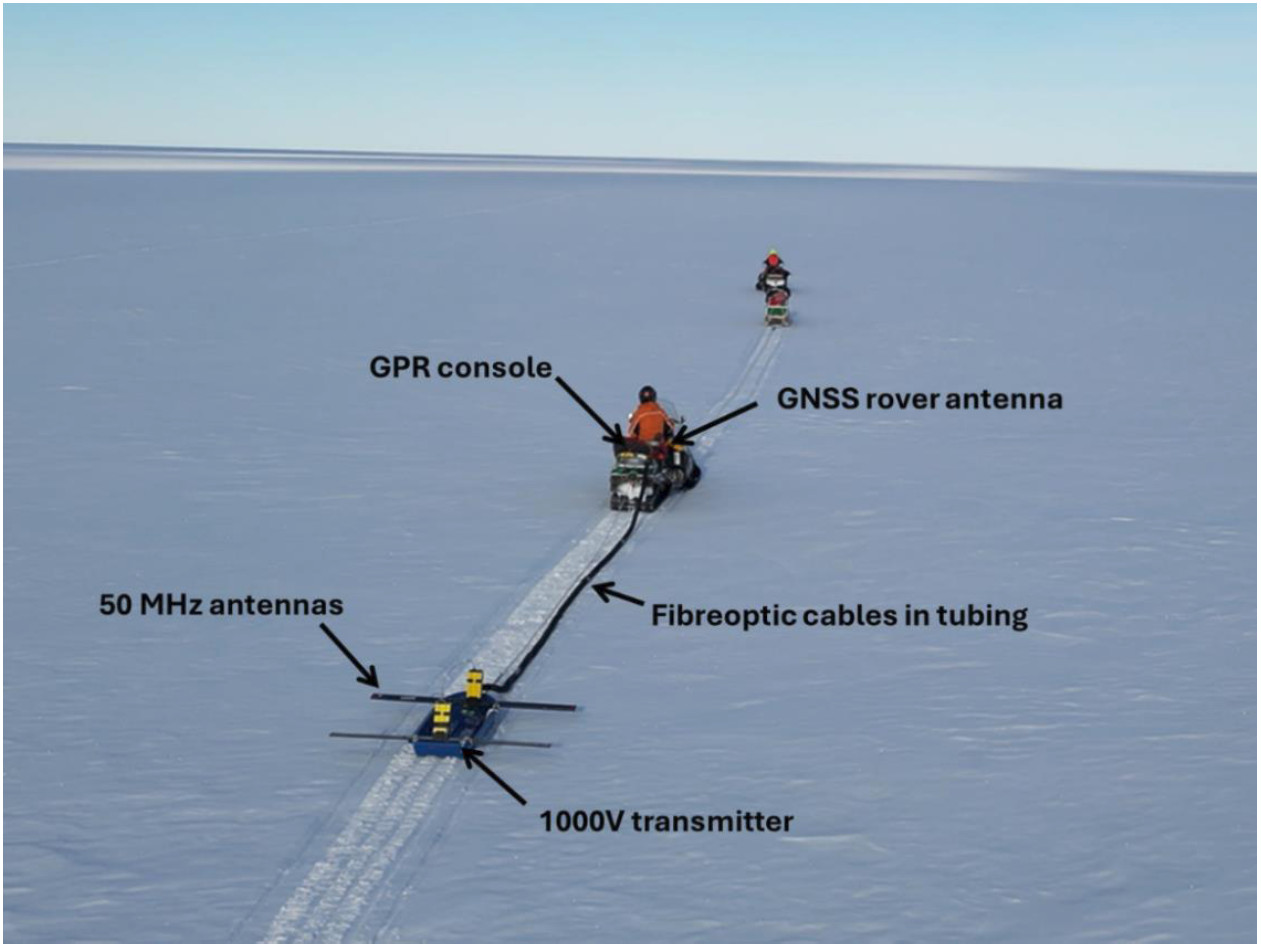
In the bistatic configuration, the dipole antennas were then mounted in the common perpendicular-broadside configuration (Allred, 2013²¹) on the plastic sledge with strings of cord, as was the aquarium tubing. This works particularly well if small holes are drilled below the upper rim of the sledge, to feed the cord through. In this case, the dimensions of the small plastic sledge limited the transmitter and receiver antenna separation to 1.4 m. We tested a range of antennas as well as the multichannel adapter, but akin to previous surveys on the LCIS, concluded that the 50 MHz antennas with the 1000 V transmitter provide data sets that are ideal for our purposes of imaging the ice-shelf base as well as internal layering (see examples below). Similarly, we tested once again a range of different settings but eventually adopted our previously used settings, i.e. a sampling interval of 1.2 ns with each trace representing a distance-average stack of eight individual traces, resulting in an average trace spacing of ~2.5 m at the towing speed of ~12 km h^-1. Precise (±0.1 m) planimetric location of each trace was achieved with the Leica VIVA GS10 Professional GNSS receiver, mounted on the snowmobile (Fig. 3). Using the GEF-supplied Leica GeoOffice software, the GNSS data were post-processed in kinematic mode against a fixed base station mounted on the GEF-supplied tripod in a sheltered area in our camp, at location JP-21 (Fig. 1). The GEF-supplied instructions for connecting the GNSS and GPR systems together were very helpful in this regard.

Data quality

Transient Electromagnetics (TEM)

Figure 4. Representative TEM data following initial processing, as explained in the text below, together with forward models as also explained (Killingbeck et al., in review⁷). a 1D resistivity model of the LCIS with no basal marine ice layer (a 2 layer model: model 1). b 1D resistivity model of the LCIS with a 45 m thick, 8m basal marine ice layer (a 3-layer model: model 2). c comparison of the data fit to model 1 (a) and model 2 (b) showing model 2 has the best fit to the observed data. The red points show the background noise.

Ground-penetrating radar (GPR)

Figure 5. Following processing as explained below, data quality was similarly excellent to previous surveys with the Sensors & Software PE PRO GPR system on the Larsen C Ice Shelf (LCIS). This is illustrated here by clear englacial layering close to borehole SI-47 (see Fig. 1 for location), whose strike and dip matches that recorded in a number of ice units identified by optical televiewing in the borehole (Miles et al., accepted²²). In Unit 4, englacial layer dip is so pronounced that coherency of radar energy return to the surface is lost. A more spatially extensive radargram, including iceshelf basal reflections and those from an englacial brine layer in a suture zone, is shown in Fig. 6b.

As the GEF-Edinburgh staff are aware, the electronic download module in the Sensors & Software console unfortunately broke early on during our fieldwork. Given it was our only Antarctic field season for the RIP-ICE project, the field team agreed that it was worth the risk to spend a considerable amount of time acquiring our planned longline and high-resolution GPR grids (Fig. 1), and storing the data on the console only; in the hope that the data could be recovered later by the manufacturer. Unfortunately this was not the case, and a large percentage of the data actually acquired was lost as the manufacturer was unable to recover them. Given that Antarctic fieldwork opportunities like this cannot easily be replicated, it is worth safeguarding against such problems by bringing appropriate spares. In our case, we had available a state of the science Mala system with ProEx console and RTA as well as paddle antennas. However, the Mala transmitter is much less powerful than the Sensors & Software 1000 V transmitter and data quality consequently rather inferior.

Processing and modelling

Transient Electromagnetics (TEM)

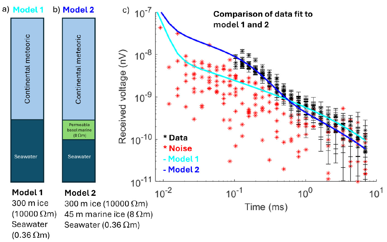
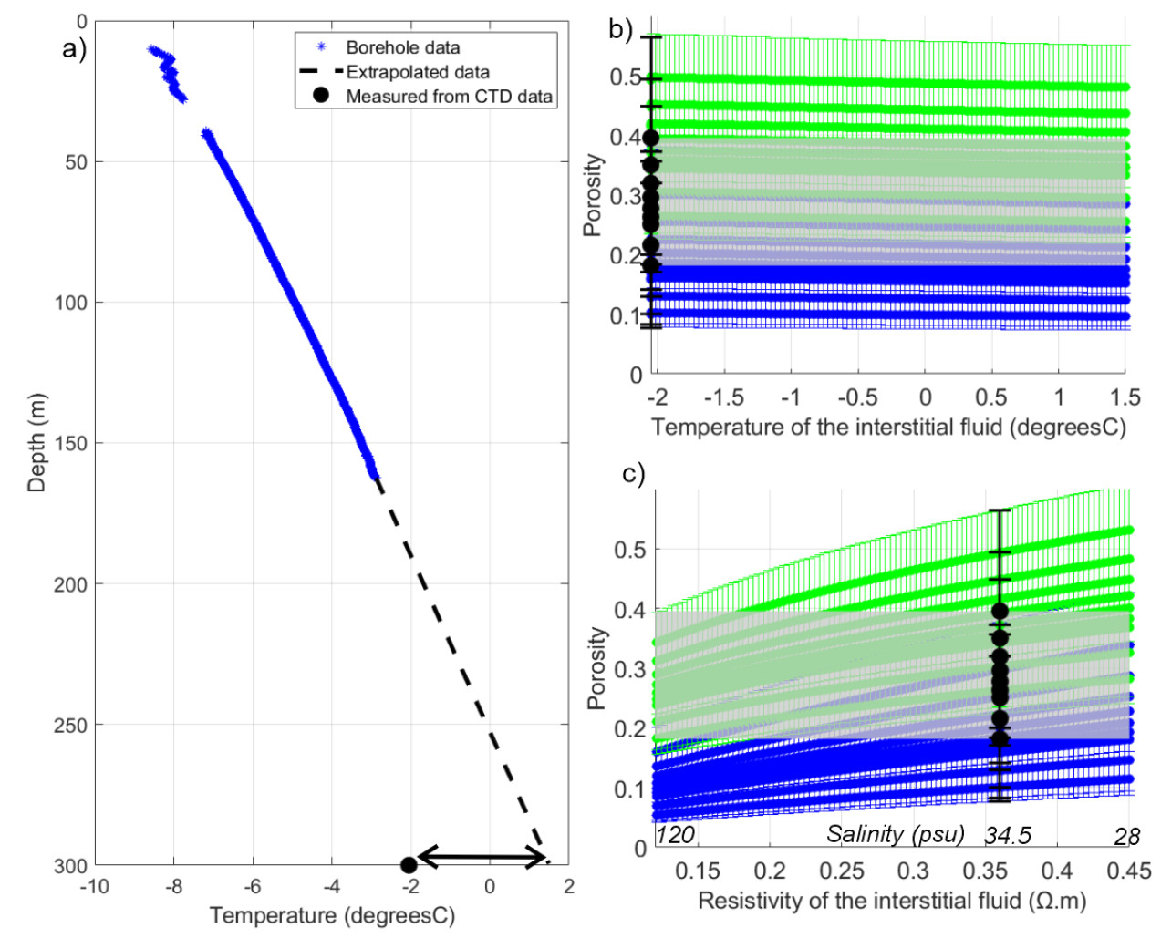
Records of magnitude below background noise (measured at each site with the transmitter coil turned off, see e.g. Fig. 4 for example) were rejected. The positive TEM data for a normal decay curve were inverted to give an estimate of the resistivity and thickness of meteoric ice and basal marine ice. We applied the open-source MATLAB code MuLTI-TEM (Killingbeck et al., 2020⁹) to invert the data using a trans-dimensional Bayesian inversion technique, which calculates the posterior probability density function of resistivity with respect to depth for each 1-D sounding (Killingbeck et al., 2020⁹). This Bayesian inversion method typically selects a simple model, such as thick layers with minimal resistivity variations, unless additional geophysical data are provided as constraints. Therefore, we apply a constrained inversion, where the sub-shelf ocean half space is constrained at 0.36 Ωm, calculated from the CTD data acquired at the Southern site reported in Nicholls et al. (2012)¹⁷: with salinity 34.54 psu, temperature -2.05 °C, and pressure 300 dBars. The inversion parameters used in MuLTI-TEM are shown in Table 1.

Table 1. TEM parameters used in MuLTI TEM

The spatially variable porosities of the permeable basal marine ice layer are estimated from bulk electrical resistivity using Archie’s Law (Archie, 1942²³). Archie’s law is commonly used to derive the relationship between porosity and resistivity in porous sedimentary rocks, and should equally apply to SIPLs (Haas et al., 1997²⁴; Hunkeler et al., 2016¹⁰) and glacier ice (Keller and Frischknecht, 1960²⁵; Kulessa, 2007¹⁶; Killingbeck et al., 2022²⁶). Here, we use Archie’s law to convert the estimated resistivity of the bulk permeable basal marine ice layer (R_m) to porosity (φ), as

$$\varphi ={\left(\frac{\alpha R_{\mathrm{s}}}{S{R}_{\mathrm{m}}}\right)}^{\frac{1}{m}}$$

where, R_s is the resistivity of the interstitial fluid in the permeable marine ice, set to the resistivity of seawater 0.36 Ωm (Nicholls et al., 2012¹⁷), m is the cementation factor assumed to range between m = 1.75 (Haas et al., 1997²⁴) and m = 3 (Hunkeler et al., 2016¹⁰), and the tortuosity factor (α) and saturation exponent (S) are set to 1 (e.g. Kovacs and Morey, 1986²⁷). It is noted that the resistivity of the interstitial fluid is unknown and could be lower than that of the underlying seawater. This is due to the exclusion of salts during ice formation, which concentrates them in the interstitial fluid, increasing its salinity and consequently lowering its resistivity.

Ground-penetrating radar (GPR)

The raw GPR data were processed using standard techniques implemented in the commercial Reflex-W package, including frequency filters, correction for energy decay, background removal, Stolt (f-k) migration (only in Fig. 5), 2-D mean filter and analytical envelope (only in Fig. 6b). Travel times were converted to depth assuming a depth-averaged radar velocity of 0.175 m ns^-1, consistent with previous estimates from common-midpoint (CMP) data (Kulessa et al., 2014³, 2019⁴).

Interpretation to date

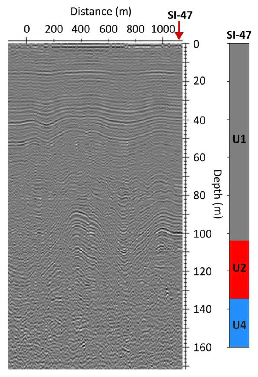
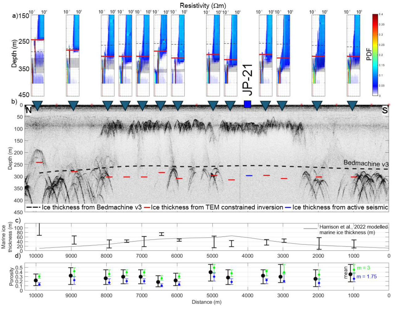
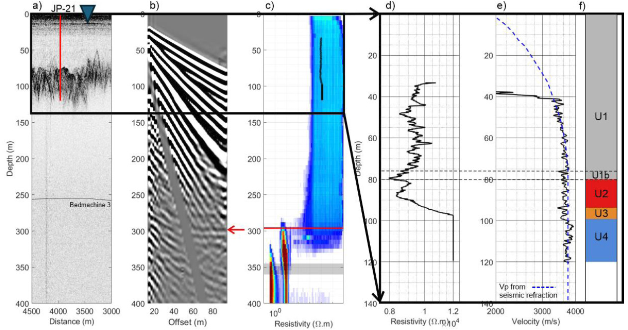
Outside the suture zone, the GPR data are characterised by multiple diffraction hyperbolas from the base of the ice shelf at thicknesses between ~300 m and ~350 m (Fig. 6b). At the 10 km position, a basal crevasse is observed extending upwards to 200 m depth. Comparing the depth of the hyperbolas’ apexes in the radargram with the ice thicknesses derived from BedMachine v3 (Morlighem et al., 2020²⁸), we find that the latter underestimates the ice thickness along this line by up to ~50 m (Fig. 6b). Inside the suture zone, the GPR data are characterised by multiple shallow diffraction hyperbolas at an average depth of ~75 m, and the base of the ice shelf is not visible. The borehole resistivity log is marked by a decrease from 9500 Ωm to 8000 Ωm through this shallow layer (Fig. 7d).

A three-layer model fits the data best in our TEM inversions, with the upper layer characterised by resistivities ranging between 1000 m and 1 000 000 m (Figs 4 and 6a). This range encompasses the values measured by our borehole resistivity log (Fig. 7c), although the inverted TEM data do not resolve the resistivity decrease (from 9500 Ωm to 8000 Ωm) shown at ~75 m depth. These data are only sensitive to changes in resistivity when the bulk resistivity is < ~1000 Ωm.

We pick the depth of the upper layer from the constrained TEM inversion, 300 m ±10 m, excluding the TEM measurement over the basal crevasse at the 10 km position (Fig. 6a). The picked depths of the upper layer match closely those of the diffraction hyperbolas in the radargram at the base of the ice shelf (Fig. 6b). Beneath this resistive upper layer, we detect an intermediate conductor characterised by resistivities of 3 Ωm - 20 Ωm (Fig. 6a). The depth of the base of the intermediate conductor is picked from the constrained TEM inversion. However, the data points associated with the base of the intermediate conductor are close to levels of background noise (Fig. 4), thus it is difficult to pick an exact depth to the lower layer. Therefore, a depth range is picked and the thickness of the intermediate conductor is estimated by subtracting the depth of the upper layer from the depth range picked, giving a 25 m to 56 m thick layer (Fig. 6c). Finally, the lower layer is the constrained seawater half space (0.36 Ωm).

Figure 6. a Constrained TEM inversion results. b Processed radargram (showing the analytical envelope) with TEM station locations shown by the blue triangles. c Estimated basal marine ice thickness along the radar line. d Estimated porosity of the basal marine ice layer along the radar line, green error bars are porosities derived with m = 3, blue error bars are porosities derived with m = 1.75 and black error bars are the mean. In a and b, the depth of the resistive upper layer, picked from the TEM, is highlighted by the red lines. The black dotted line is the ice thickness derived from BedMachine v3 (Morlighem et al., 2020²⁸). In a, the estimated depth of the transition to seawater is highlighted by the grey box. In b, the depth of the observed seismic reflection (Fig. 7b) is highlighted by the blue line.

The common-offset stacked seismic data image a weak negative reflector (black-white-black) at a TWT of 0.167 s (Fig. 7b). The P-wave velocity profile derived in Kulessa et al. (2019)⁴: agrees closely with the borehole sonic log (Fig. 7e) and is used to convert the TWT of the common offset stack to depth, where the weak negative reflector occurs at a depth of ~297 m (Fig. 7b). This depth matches closely with that of the resistive upper layer picked from the TEM constrained inversions (296 m) next to JP-21 (Figs 6b and Fig. 7c).

Figure 7. a Zoomed in section around JP-21 (see Fig. 1 for location) of the processed radargram, showing the analytical envelope. b Seismic common offset stacked data in depth. The red arrow highlights the observed negative polarity reflection (black-white-black), where the polarity of the direct wave (defining a positive polarity) is white-black-white. c Constrained TEM inversion result of the sounding next to JP-21 with the electrical resistivity log plotted (black line). d Electrical resistivity log. e Sonic log (black line) and Vp profile derived in Kulessa et al., 2019⁴ (blue dashed line). f Optical televiewer interpreted units 1 - 4 (U1 - U4) plotted adjacent to the borehole wireline logs reported in Miles at al. (accepted)²², with unit 1b (U1b) picked in this study.

Preliminary findings

Properties of the basal marine ice layer

The GPR, TEM and seismic data are all consistent with the presence of an interface at ~300 m depth. This interface is characterised by a large decrease in resistivity (from ~1000 Ωm - ~1 000 000 Ωm to 3 Ωm - 20 Ωm) and a decrease in acoustic impedance as indicated by the negative polarity wavelet of seismic basal reflection. We interpret this interface to be a transition from meteoric ice, or potentially impermeable marine ice (Craven et al., 2009¹⁴) with electrical properties in the range 1000 Ωm - 1 000 000 Ωm, to permeable basal marine ice that corresponds to the intermediate conductor delineated by the inversion results (Fig. 6a). The TEM-derived basal marine ice thicknesses are on the same order of magnitude as those modelled by Harrison et al. (2022)⁶: (Fig. 6c), except in the presence of basal crevasses where they significantly differ (e.g. at the 10 km position of the GPR line the difference is ~80 m; Figs 6b and 6c). This highlights the importance of field measurements over model assumptions.

The resistivity values of the basal marine ice layer are picked from the TEM data and converted to porosity using Equation 1. The mean estimated porosities along the profile range from 0.18 - 0.40 (Fig. 6d). Acknowledging that the interstitial fluid resistivity (R_s) could be lower than the seawater resistivity used in our porosity calculations (Equation 1), and that the temperature may deviate from the assumed -2.05 °C, we performed a sensitivity analysis. Utilizing temperature data from JP-21, extrapolated to 300 m depth, we estimated an upper temperature bound of 1.5 °C (Fig. 8a) for this analysis. Systematically varying the temperature from -2.05 °C to 1.5 °C resulted in a negligible impact on our reported porosity range (Fig. 8b). Similarly, we estimate the upper bound using a salinity of 120 psu, when solid precipitates start to form in seawater changing its composition (Sharqawy et al., 2010²⁹), this gives an of 0.12 Ωm. By systematically varying from 0.12 Ωm to 0.45 Ωm (Fig. 8c), the analysis demonstrates that our reported range sufficiently accounts for variations in . Notably, a minimum of 0.12 Ωm, would yield a lower mean porosity range of 0.12-0.25 (Fig. 8c), comparable to the 0.14-0.20 range estimated at the Amery Ice Shelf (Craven et al., 2009¹⁴). However, this high salinity is only likely in a brine drainage scenario near the upper part of the marine ice matrix and not representative of the bulk marine ice properties.

Figure 8. a Borehole temperature profile from JP-21 (see Fig. 1 for location). Sensitivity analysis of porosity with varying b temperature and c interstitial fluid resistivity for all TEM locations. Green error bars are porosities derived with m = 3, blue error bars are porosities derived with m = 1.75 and black error bars are the mean porosities reported with temperature -2.05 °C and R_s = 0.36 m (with the grey background fill).

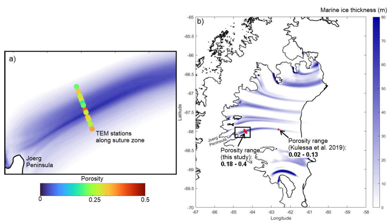
Comparing our porosity estimates with a site 195 km downstream LCIS, our estimates are significantly larger than those estimated by Kulessa et al. (2019)⁴, 0.02 - 0.13, for this downstream location (Fig. 9). Our inferences of porosity ranges are therefore consistent with basal marine ice compaction along the suture zone (Fig. 9b). Compaction reduces both the overall thickness and the seawater content of the basal marine ice, which exerts the strongest control on its ability to arrest rifts (Kulessa et al., 2019⁴). This ability is therefore likely largest at an unknown intermediate location along the suture zone where basal marine ice thickness and seawater content are greatest, relative to the thickness of meteoric ice prone to brittle fracture. That ability will then decrease towards the calving front as the marine ice progressively compacts, which may have implications for the future stability of the LCIS if basal melting increases in a warming sub-shelf ocean cavity (Kulessa et al., 2014³; McGrath et al., 2014³⁰).

Figure 9. a Modelled basal marine ice thicknesses of the LCIS from Harrison et al. (2022)⁶, compared to this study’s estimated porosities from our TEM data, and b estimated porosity in Kulessa et al., 2019⁴ at the downstream location -67.953555°, -62.623506°.

Conclusions and recommendations

We have shown that TEM methods are capable of detecting and characterizing permeable basal marine ice in suture zones, which has proven to be difficult with conventional geophysical methods. We show that TEM can estimate the thickness of meteoric ice and the resistivity and thickness of the basal marine ice layer beneath our study site on LCIS. TEM methods provide a resistivity-depth profile, resolving the vertical resistivity structure of the subsurface. This is different from frequency domain EM methods, which have been successfully used to detect and quantify SIPL beneath sea ice, where their high signal-to-noise ratios make them sensitive to lateral variations in conductivity, rather than vertical changes with depth. Thus, the novel use of TEM to characterize basal marine ice is appropriate for resolving its vertical structure and determining its thickness, key parameters in understanding its formation and evolution.

The depth of investigation of TEM systems is primarily controlled by the transmitter loop size and current, as detailed in Killingbeck et al. (2022²⁶). Our study demonstrates the capability of a 4 x 100 m square loop with a 2 A current to image through approximately 300 m of ice shelf. The relatively flat surface of ice shelves and the common availability of snow scooters facilitate the deployment of larger loop soundings, enabling deeper investigations. While our reported setup is effective for the ice thickness encountered, powerful ground-based TEM systems with larger loops and higher currents are available and would be necessary to image the base of thicker ice shelves. Furthermore, although not used in this study, airborne TEM systems offer an effective means of acquiring broad spatial coverage, particularly over large ice shelves, but are typically limited in their depth penetration compared to large-loop ground-based systems. Borehole logging and sampling offer high-resolution insights into marine ice properties, but are inherently limited by their point-source nature and require extensive time investment. Thus, integrating borehole measurements with spatially distributed TEM data would allow us to overcome this limitation. The TEM data would enable interpolation of the borehole measurements, effectively extending information across the entire suture zone.

References

1. Craw, L (2023). The influence of marine ice on ice shelf dynamics and stability. University of Tasmania. Thesis. ↩

2. Khazendar A, Rignot E and Larour E (2009) Roles of marine ice, rheology, and fracture in the flow and stability of the Brunt/Stancomb-Wills Ice Shelf. Journal of Geophysical Research: Earth Surface 114(4), 1 9. https://doi.org/10.1029/2008JF001124 ↩

3. Kulessa, B., Jansen, D., Luckman, A. J., King, E. C., & Sammonds, P. R. (2014). Marine ice regulates the future stability of a large Antarctic ice shelf. Nature Communications, 5(1), 3707. https://doi.org/10.1038/ncomms4707 ↩ ↩² ↩³ ↩⁴ ↩⁵

4. Kulessa, B., Booth, A. D., O’Leary, M., McGrath, D., King, E. C., Luckman, A. J., … & Hubbard, B. (2019). Seawater softening of suture zones inhibits fracture propagation in Antarctic ice shelves. Nature Communications, 10(1), https://doi.org/10.1038/s41467-019-13539-x ↩ ↩² ↩³ ↩⁴ ↩⁵ ↩⁶ ↩⁷ ↩⁸ ↩⁹

5. Jansen, D., Luckman, A. J., Cook, A., Bevan, S., Kulessa, B., Hubbard, B., & Holland, P. R. (2015). Brief Communication: Newly developing rift in Larsen C Ice Shelf presents significant risk to stability. The Cryosphere, 9(3), 1223-1227. https://doi.org/10.5194/tc-9-1223-2015 ↩

6. Harrison, L. C., Holland, P. R., Heywood, K. J., Nicholls, K. W., & Brisbourne, A. M. (2022). Sensitivity of melting, freezing and marine ice beneath Larsen C Ice Shelf to changes in ocean forcing. Geophysical Research Letters, 49(4), e2021GL096914. https://doi.org/10.1029/2021GL096914 ↩ ↩² ↩³

7. Killingbeck, S. F., B. Kulessa, K. E. Miles, B. Hubbard, A. Luckman, S. S. Thompson, G. Jones, B. K. Galton-Fenzi. Transient electromagnetic imaging of permeable marine ice at the base of Larsen C Ice Shelf, Antarctic Peninsula. Geophysical Research Letters, in review. ↩ ↩²

8. Mikucki, J. A., Auken, E., Tulaczyk, S., Virginia, R. A., Schamper, C., S rensen, K. I., … & Foley, N. (2015). Deep groundwater and potential subsurface habitats beneath an Antarctic dry valley. Nature communications, 6(1), 6831. https://doi.org/10.1038/ncomms7831 ↩

9. Killingbeck, S. F., Booth, A. D., Livermore, P. W., Bates, C. R., & West, L. J. (2020). Characterisation of subglacial water using a constrained transdimensional Bayesian transient electromagnetic inversion. Solid Earth, 11(1), 75-94. https://doi.org/10.5194/se-11-75-2020 ↩ ↩² ↩³

10. Hunkeler, P. A., Hoppmann, M., Hendricks, S., Kalscheuer, T., & Gerdes, R. (2016). A glimpse beneath Antarctic sea ice: Platelet layer volume from multifrequency electromagnetic induction sounding. Geophysical Research Letters, 43(1), 222 231. https://doi.org/10.1002/2015GL065074 ↩ ↩² ↩³

11. Brett, G. M., Irvin, A., Rack, W., Haas, C., Langhorne, P. J., & Leonard, G. H. (2020). Variability in the Distribution of Fast Ice and the Sub-ice Platelet Layer Near McMurdo Ice Shelf. Journal of Geophysical Research: Oceans, 125, e2019JC015678. https://doi.org/10.1029/2019JC015678 ↩

12. Haas, C., Langhorne, P. J., Rack, W., Leonard, G. H., Brett, G. M., Price, D., … & Gough, A. J. (2021). Airborne mapping of the sub-ice platelet layer under fast ice in McMurdo Sound, Antarctica. The Cryosphere, 2020, 1 31. https://doi.org/10.5194/tc-15-247-2021, 2021. ↩ ↩²

13. Craven M, Carsey F, Behar A, et al. Borehole imagery of meteoric and marine ice layers in the Amery Ice Shelf, East Antarctica. (2005) Journal of Glaciology. 2005;51(172):75-84. https://doi.org/10.3189/172756505781829511 ↩

14. Craven, M., Allison, I., Fricker, H. A., & Warner, R. (2009). Properties of a marine ice layer under the Amery Ice Shelf, East Antarctica. Journal of Glaciology, 55(192), 717-728. https://doi.org/10.3189/002214309789470941 ↩ ↩² ↩³

15. Craven M, Warner RC, Galton-Fenzi BK, Herraiz-Borreguero L, Vogel SW, Allison I. (2014) Platelet ice attachment to instrument strings beneath the Amery Ice Shelf, East Antarctica. Journal of Glaciology. 60(220):383-393. https://doi.org/10.3189/2014JoG13J082 ↩

16. Kulessa, B. (2007). A critical review of the low-frequency electrical properties of ice sheets and glaciers. Journal of Environmental & Engineering Geophysics, 12(1), 23-36. https://doi.org/10.2113/JEEG12.1.23 ↩ ↩²

17. Nicholls, K. W., Makinson, K., & Venables, E. J. (2012). Ocean circulation beneath Larsen C Ice Shelf, Antarctica from in situ observations. Geophysical Research Letters, 39(19). https://doi.org/10.1029/2012GL053187 ↩ ↩² ↩³

18. Gough, A. J., Mahoney, A. R., Langhorne, P. J., Williams, M. J. M., & Haskell, T. G. (2012). Sea ice salinity and structure: A winter time series of salinity and its distribution. J. Geophys. Res.-Oceans, 117(C3). https://doi.org/10.1029/2011JC007527 ↩

19. Langhorne, P. J., Hughes, K. G., Gough, A. J., Smith, I. J., Williams, M. J. M., Robinson, N. J., … & Haskell, T. G. (2015). Observed platelet ice distributions in Antarctic sea ice: An index for oceanice shelf heat flux. Geophysical Research Letters, 42(13), 5442-5451. https://doi.org/10.1002/2015GL064508 ↩

20. Haran, T., Klinger, M., Fahnestock, M., Painter, T. & Scambos, T. (2018) MEaSUREs MODIS Mosaic of Antarctica 2013-2014 (MOA2014) Image Map, Version 1. NASA National Snow and Ice Data Center Distributed Active Archive Center Preprint at https://doi.org/10.5067/RNF17BP824UM. ↩

21. Allred, B. J. (2013). A GPR Agricultural Drainage Pipe Detection Case Study: Effects of Antenna Orientation Relative to Drainage Pipe Directional Trend. Journal of Environmental and Engineering Geophysics, 18(1), 55-69. https://doi.org/10.2113/jeeg18.1.55 ↩

22. Miles, K. E., Hubbard, B., Luckman, A., Kulessa, B., Bevan. S., Thompson, S., and Jones, G. Influence of the grounding zone on the internal structure of ice shelves. Nature Communications, accepted. ↩ ↩²

23. Archie, G.E. (1942) The Electrical Resistivity Log as an Aid in Determining Some Reservoir Characteristics. Transactions of the AIME, 146, 54-62. ↩

24. Haas, C., Gerland, S., Eicken, H., & Miller, H. (1997). Comparison of sea-ice thickness measurements under summer and winter conditions in the Arctic using a small electromagnetic induction device. Geophysical Research Letters, 62(3), 749 757. https://doi.org/10.1190/1.1444184 ↩ ↩²

25. Keller, G. V., & Frischknecht, F. C. (1960). Electrical resistivity studies on the Athabasca glacier, Alberta, Canada. Journal of Research of the National Bureau of Standards D, 64, 439-448. ↩

26. Killingbeck, S. F., Dow, C. F., & Unsworth, M. J. (2022). A quantitative method for deriving salinity of subglacial water using ground-based transient electromagnetics. Journal of Glaciology, 68(268), 319-336. https://doi.org/10.1017/jog.2021.94 ↩ ↩²

27. Kovacs, A., & Morey, R. M. (1986). Electromagnetic measurements of multi-year sea ice using impulse radar. Cold Regions Science and Technology, 12(1), 67-93. ↩

28. Morlighem, M., Rignot, E., Binder, T., Blankenship, D., Drews, R., Eagles, G., … & Young, D. A. (2020). Deep glacial troughs and stabilizing ridges unveiled beneath the margins of the Antarctic ice sheet. Nature Geoscience, 13(2), 132-137. ↩ ↩²

29. Sharqawy, M. H., Lienhard, J. H., & Zubair, S. M. (2010). Thermophysical properties of seawater: a review of existing correlations and data. Desalination and Water Treatment, 16(1-3), 354-380. https://doi.org/10.5004/dwt.2010.1079 ↩

30. McGrath, D., Steffen, K., Holland, P. R., Scambos, T., Rajaram, H., Abdalati, W., & Rignot, E. (2014). The structure and effect of suture zones in the Larsen C Ice Shelf, Antarctica. Journal of Geophysical Research: Earth Surface, 119(3), 588-602. https://doi.org/10.1002/2013JF002935 ↩